- Instructions for R are here: http://epsy887.bryer.org/getting_started/software/
LaTeX
install.packages('tinytex')
tinytex::install_tinytex()
August 29, 2019
install.packages('tinytex')
tinytex::install_tinytex()
Open the R/setup.R file in RStudio and click the Source button.
Or run this command in R:
source('https://raw.githubusercontent.com/jbryer/IntroR/master/Installation/Setup.r')
This is the contents of that R script:
pkgs <- c('tidyverse','devtools','reshape2','RSQLite',
          'psa','multilevelPSA','PSAboot','TriMatch','likert',
          'openintro','OIdata','psych','knitr','markdown','rmarkdown','shiny')

install.packages(pkgs)

devtools::install_github('jbryer/ipeds')
devtools::install_github('jbryer/sqlutils')
devtools::install_github("seankross/lego")
devtools::install_github("jbryer/DATA606")
“R is a language and environment for statistical computing and graphics. It is a GNU project which is similar to the S language and environment which was developed at Bell Laboratories (formerly AT&T, now Lucent Technologies) by John Chambers and colleagues…”
“R provides a wide variety of statistical (linear and non linear modeling, classical statistical tests, time-series analysis, classification, clustering, …) and graphical techniques, and is highly extensible. The S language is often the vehicle of choice for research in statistical methodology, and R provides an Open Source route to participation in that activity.”
(R-project.org)
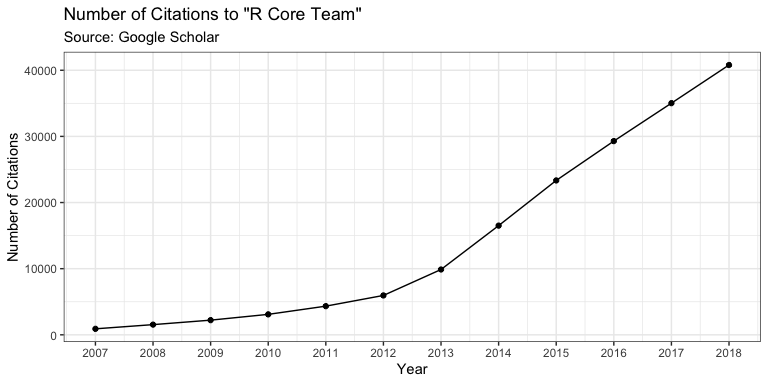
Firth, D (2011). R and citations. Weblog entry at URL https://statgeek.wordpress.com/2011/06/25/r-and-citations/.
See also: Muenchen, R.A. (2017). The Popularity of Data Analysis Software. Welog entry at URL http://r4stats.com/articles/popularity/
In “Stages in the Evolution of S”, John Chambers writes:
“[W]e wanted users to be able to begin in an interactive environment, where they did not consciously think of themselves as programming. Then as their needs became clearer and their sophistication increased, they should be able to slide gradually into programming, when the language and system aspects would become more important.”
The latest version of R can be downloaded from cran.r-project.org. The current version of R is:
R.version$version.string
## [1] "R version 3.6.1 (2019-07-05)"
You will also want to install RStudio.
Installation instructions are available here: http://epsy887.bryer.org/getting_started/software/
To install the set of packages used for this workshop, run the following R command:
source('https://raw.githubusercontent.com/jbryer/EPSY887Fall2019/master/R/Setup.r')
2 + 2
## [1] 4
1 + sin(9)
## [1] 1.412118
exp(1) ^ (1i * pi)
## [1] -1+0i
\[ { e }^{ i\pi }+1=0 \]
“The most remarkable formula in mathematics”
- Richard Feyneman
One aspect that makes R popular is how (relatively) easy it is to extend it’s functionality vis-à-vis R packages. R packages are collections of R functions, data, and documentation.
The Comprehensive R Archive Network (CRAN) is the central repository where R packages are published. However, it should be noted that there are mirrors located across the globe.
Using packages requires two steps: first, install the package (required once per R installation); and second, load the package (once per R session).
install.packages('likert')
library(likert)
The library() function without any parameters will print all installed R packages whereas the search() function will list loaded packages (technically all available namespaces/environments, more on that later).
library()
search()
##  [1] ".GlobalEnv"        "package:likert"    "package:xtable"    "package:scholar"
##  [5] "package:lubridate" "package:forcats"   "package:stringr"   "package:purrr"
##  [9] "package:readr"     "package:tidyr"     "package:tibble"    "package:tidyverse"
## [13] "package:dplyr"     "package:ggplot2"   "package:stats"     "package:graphics"
## [17] "package:grDevices" "package:utils"     "package:datasets"  "package:methods"
## [21] "Autoloads"         "package:base"
Github is an online source repository and has become a popular place for R package developers to store their R packages. The devtools R package, designed to help package developers, has a function, install_github that will install R packages from a Github repository.
devtools::install_github('jbryer/likert')
ls()We can use the ls() function to determine what functions are available in a package.
ls('package:likert')
## [1] "likert"                "likert.bar.plot"       "likert.density.plot"   "likert.heat.plot"
## [5] "likert.histogram.plot" "likert.options"        "recode"                "reverse.levels"
R provides extensive documentation and help. The help.start() function will launch a webpage with links to: * The R manuals * The R FAQ * Search engine * and many other useful sites
The help.search() function will search the help file for a particular word or phrase. For example:
help.search('cross tabs')
To get documentation on a specific function, the help() function, or simply ?functionName will open the documentation page in the web browser.
Lastly, to search the R mailing lists, use the RSiteSearch() function.
| Data File Type | Extension | Function |
|---|---|---|
| R Data | rda, rdata | base::load, base::readRDS |
| Comma separated values | csv | utils::read.csv, readr::read_csv |
| Other delimited files | utils::read.table, readr::read_delim |
|
| Tab separated files | readr::read_tsv |
|
| Fixed width files | utils::read.fwf, readr::read_fwf |
|
| SPSS | sav | foreign::read.spss, haven::read_sav, haven::read_por |
| SAS | sas | haven::read_sas |
| Read lines | base::scan, readr::read_lines |
|
| Microsoft Excel | xls, xlsx | gdata::read.xls, readxl::read_excel |
The RODBC package is the most common way to connect to a variety of databases.
odbcConnect - Open a connection to an ODBC databasesqlFetch - Read a table from an ODBC database into a data framesqlQuery - Submit a query to an ODBC database and return the resultsclose - Close the connectionOther packages used to connect to specific databases:
RMySQLROracleRJDBCRSQLiteRPosgreSQLsqlutils PackageThe sqlutils is designed to help manage many query files and facilitates documenting and parameterizing the queries.
library(sqlutils)
sqlPaths()
## [1] "/Library/Frameworks/R.framework/Versions/3.6/Resources/library/sqlutils/sql"
getQueries()
## [1] "StudentsInRange" "StudentSummary"
getParameters('StudentsInRange')
## [1] "startDate" "endDate"
StudentsInRange)#' Students enrolled within the given date range. #' #' @param startDate the start of the date range to return students. #' @default startDate format(Sys.Date(), '%Y-01-01') #' @param endDate the end of the date range to return students. #' @default endDate format(Sys.Date(), '%Y-%m-%d') #' @return CreatedDate the date the row was added to the warehouse data. #' @return StudentId the student id. SELECT * FROM students WHERE CreatedDate >= ':startDate:' AND CreatedDate <= ':endDate:'
sqldoc('StudentsInRange')
## Students enrolled within the given date range.
## Parameters:
##      param                                            desc                        default
##  startDate the start of the date range to return students.                   '2012-01-01'
##    endDate   the end of the date range to return students. format(Sys.Date(), '%Y-%m-%d')
##  default.val
##   2012-01-01
##   2019-08-29
## Returns (note that this list may not be complete):
##     variable                                              desc
##  CreatedDate the date the row was added to the warehouse data.
##    StudentId                                   the student id.
require(RSQLite)
sqlfile <- paste(system.file(package='sqlutils'), '/db/students.db', sep='')
m <- dbDriver("SQLite")
conn <- dbConnect(m, dbname=sqlfile)
q1 <- execQuery('StudentSummary', connection=conn)
head(q1)
##   CreatedDate count
## 1  2011-07-15  2886
## 2  2011-08-15  2983
## 3  2011-09-15  3071
## 4  2011-10-15  3059
## 5  2011-11-15  3058
## 6  2011-12-15  3074
The ipeds R package provides an interface to download data file from IPEDS.
library(ipeds)
data(surveys)
unique(surveys$Survey)
##  [1] Institutional Characteristics       Enrollments
##  [3] Completions                         Instructional staff/Salaries
##  [5] Fall Staff                          Employees by Assigned Position
##  [7] Finance                             Graduation Rates
##  [9] Student Financial Aid and Net Price Admission and Test Scores
## [11] Admissions                          12-month Enrollment
## [13] Fall Enrollment                     Outcome Measures
## [15] Human Resources                     Academic Libraries
## 16 Levels: Admission and Test Scores Completions Employees by Assigned Position ... Academic Libraries
head(surveys[,c('SurveyID','Title')])
##   SurveyID                                                                               Title
## 1       HD                                                               Directory information
## 2       IC Educational offerings, organization, admissions, services and athletic associations
## 3    IC_AY                                          Student charges for academic year programs
## 4    IC_PY                                    Student charges by program (vocational programs)
## 5    FLAGS                                           Response status for all survey components
## 6    EFEST                                                                Estimated enrollment
The getIPEDSSurvey and ipedsHelp are the most commonly used functions. The former will download and load the data into R (note data is cached and downloaded once per installation); the latter will provide the data dictionary for the given survey.
directory = getIPEDSSurvey('HD', 2013)
admissions = getIPEDSSurvey("IC", 2013)
retention = getIPEDSSurvey("EFD", 2013)
ipedsHelp('HD', 2013)
head(directory)
##   unitid                              instnm                           addr       city stabbr
## 1 100654            Alabama A & M University           4900 Meridian Street     Normal     AL
## 2 100663 University of Alabama at Birmingham Administration Bldg Suite 1070 Birmingham     AL
## 3 100690                  Amridge University                 1200 Taylor Rd Montgomery     AL
## 4 100706 University of Alabama in Huntsville                301 Sparkman Dr Huntsville     AL
## 5 100724            Alabama State University           915 S Jackson Street Montgomery     AL
## 6 100733 University of Alabama System Office             401 Queen City Ave Tuscaloosa     AL
##          zip fips obereg                  chfnm   chftitle      gentele    faxtele       ein
## 1      35762    1      5 Dr. Andrew Hugine, Jr.  President 2.563725e+09 2563725030 636001109
## 2 35294-0110    1      5           Ray L. Watts  President 2.059344e+09 2059757114 636005396
## 3 36117-3553    1      5         Michael Turner  President 3.343877e+13 3343873878 237034324
## 4      35899    1      5   Robert A. Altenkirch  President 2.568246e+09         NA 630520830
## 5 36104-0271    1      5              Gwen Boyd  President 3.342294e+09 3348346861 636001101
## 6      35401    1      5            Robert Witt Chancellor 2.053490e+09 2053485206 636001138
##     opeid opeflag                        webaddr                                      adminurl
## 1  100200       1                  www.aamu.edu/    www.aamu.edu/admissions/pages/default.aspx
## 2  105200       1                    www.uab.edu www.uab.edu/students/undergraduate-admissions
## 3 2503400       1      www.amridgeuniversity.edu  www.amridgeuniversity.edu/au_admissions.html
## 4  105500       1                    www.uah.edu                           admissions.uah.edu/
## 5  100500       1 www.alasu.edu/email/index.aspx           www.alasu.edu/admissions/index.aspx
## 6  800400       2            www.uasystem.ua.edu
##                                                 faidurl
## 1 www.aamu.edu/Admissions/fincialaid/Pages/default.aspx
## 2               www.uab.edu/students/paying-for-college
## 3        www.amridgeuniversity.edu/au_financialaid.html
## 4                                       finaid.uah.edu/
## 5                    www.alasu.edu/cost-aid/index.aspx/
## 6
##                                                                                                                                          applurl
## 1                                                                                               www.aamu.edu/Admissions/apply/Pages/default.aspx
## 2                                                                                    ssb.it.uab.edu/pls/sctprod/zsapk003_ug_web_appl.create_page
## 3                                          https://www.amridgeuniversity.edu/Amridge/login.aspx?ReturnUrl=%2fAmridge%2fStudent%2fFormChoice.aspx
## 4                                                                                                                               register.uah.edu
## 5 psadmin.alasu.edu:8501/psp/paprd_1/EMPLOYEE/HRMS/c/ASU_SS_NONID_MENU.ASU_SS_ONL_SECURE.GBL?PORTALPARAM_PTCNAV=ASU_LK_ONLINEAPP&EOPP.SCNode=EMP
## 6
##                                                                                  npricurl sector
## 1                                          galileo.aamu.edu/netpricecalculator/npcalc.htm      1
## 2                                         www.collegeportraits.org/AL/UAB/estimator/agree      1
## 3 tcc.noellevitz.com/(S(miwoihs5stz5cpyifh4nczu0))/Amridge%20University/Freshman-Students      2
## 4                                                                         finaid.uah.edu/      1
## 5                                     www.alasu.edu/cost-aid/forms/calculator/index.aspx/      1
## 6                                                                     www.uasystem.ua.edu      0
##   iclevel control hloffer ugoffer groffer hdegofr1 deggrant hbcu hospital medical tribal locale
## 1       1       1       9       1       1       12        1    1        2       2      2     12
## 2       1       1       9       1       1       11        1    2        1       1      2     12
## 3       1       2       9       1       1       11        1    2        2       2      2     12
## 4       1       1       9       1       1       11        1    2        2       2      2     12
## 5       1       1       9       1       1       11        1    1        2       2      2     12
## 6       1       1       9       1       1       11        1    2        2      -2      2     13
##   openpubl act newid deathyr closedat cyactive postsec pseflag pset4flg rptmth
## 1        1  A     -2      -2       -2        1       1       1        1      1
## 2        1  A     -2      -2       -2        1       1       1        1      1
## 3        1  A     -2      -2       -2        1       1       1        1      1
## 4        1  A     -2      -2       -2        1       1       1        1      1
## 5        1  A     -2      -2       -2        1       1       1        1      1
## 6        1  A     -2      -2       -2        1       1       1        1     -2
##                                              ialias instcat ccbasic ccipug ccipgrad ccugprof
## 1                                              AAMU       2      18     13       18        9
## 2                                                         2      15     11       17        8
## 3 Southern Christian University |Regions University       2      21     11       13        6
## 4             UAH |University of Alabama Huntsville       2      15     14       17        8
## 5                                                         2      18     10       12        9
## 6                                                        -2      -3     -3       -3       -3
##   ccenrprf ccsizset carnegie landgrnt instsize  cbsa cbsatype csa necta f1systyp
## 1        4       14       16        1        3 26620        1 290    -2        2
## 2        5       15       15        2        4 13820        1 142    -2        1
## 3        5        6       51        2        1 33860        1  -2    -2        2
## 4        4       12       16        2        3 26620        1 290    -2        1
## 5        4       13       21        2        3 33860        1  -2    -2        2
## 6       -3       -3       -3        2       -2 46220        1  -2    -2        1
##                           f1sysnam f1syscod countycd          countynm cngdstcd  longitud latitude
## 1                                        -2     1089    Madison County      105 -86.56850 34.78337
## 2 The University of Alabama System   101050     1073  Jefferson County      107 -86.80917 33.50223
## 3                                        -2     1101 Montgomery County      102 -86.17401 32.36261
## 4 The University of Alabama System   101050     1089    Madison County      105 -86.63842 34.72282
## 5                                        -2     1101 Montgomery County      107 -86.29568 32.36432
## 6 The University of Alabama System   101050     1125 Tuscaloosa County      107 -87.56086 33.21252
##   dfrcgid dfrcuscg
## 1     138        1
## 2     126        1
## 3     164        2
## 4     126        2
## 5     138        1
## 6      -2       -2
+ - addition- - subtraction* - multiplication/ - division^ or ** - exponentiationx %% y - modulus (x mod y) 5%%2 is 15 %% 2
## [1] 1
x %/% y - integer division5%/%2
## [1] 2
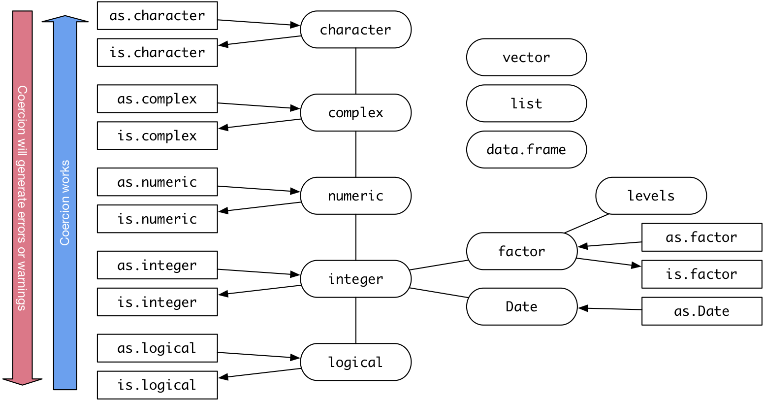
logicial (e.g. TRUE, FALSE)integer - whole numbers, either positive or negative (e.g. 2112, 42, -1)double or numeric - real number (e.g. 0.05, pi, -Inf, NaN)complex - complex number (e.g. 1i)character - sequence of characters, or a string (e.g. "Hello NEAIR!")You can use the class function to determine the type of an object.
tmp <- c(2112, pi)
class(tmp)
## [1] "numeric"
To test if an object is of a particular class, use the is.XXX set of functions:
is.double(tmp)
## [1] TRUE
And to convert from one type to another, use the as.XXX set of functions:
as.character(tmp)
## [1] "2112" "3.14159265358979"
A list is an object that contains a list of named values
tmp <- list(a = 2112, b = pi, z = "Hello EPSY887!")
tmp
## $a
## [1] 2112
##
## $b
## [1] 3.141593
##
## $z
## [1] "Hello EPSY887!"
tmp[1]; class(tmp[1]) # One square backet: return a list
## $a
## [1] 2112
## [1] "list"
tmp[[1]]; class(tmp[[2]]) # Two square brackets: return as object at that position
## [1] 2112
## [1] "numeric"
A factor is a way for R to store a nominal, or categorical, variable. R stores the underlying data as an integer where each value corresponds to a label.
gender <- c(rep("male",4), rep("female", 6))
gender
## [1] "male" "male" "male" "male" "female" "female" "female" "female" "female" "female"
gender <- factor(gender, levels=c('male','female','unknown'))
gender
##  [1] male   male   male   male   female female female female female female
## Levels: male female unknown
levels(gender)
## [1] "male" "female" "unknown"
The ordered parameter indicates whether the levels in the factor should be ordered.
library(TriMatch)
## Loading required package: scales
##
## Attaching package: 'scales'
## The following object is masked from 'package:purrr':
##
##     discard
## The following object is masked from 'package:readr':
##
##     col_factor
## Loading required package: reshape2
##
## Attaching package: 'reshape2'
## The following object is masked from 'package:tidyr':
##
##     smiths
## Loading required package: ez
## Registered S3 methods overwritten by 'lme4':
##   method                          from
##   cooks.distance.influence.merMod car
##   influence.merMod                car
##   dfbeta.influence.merMod         car
##   dfbetas.influence.merMod        car
data(tutoring, package='TriMatch')
head(tutoring$Grade)
## [1] 4 4 4 4 4 3
grade <- tutoring$Grade
table(grade, useNA='ifany')
## grade
##   0   1   2   3   4
## 187  25  86 271 573
grade <- factor(tutoring$Grade,
        levels=0:4,
        labels=c('F','D','C','B','A'),
        ordered=TRUE)
table(grade, useNA='ifany')
## grade
##   F   D   C   B   A
## 187  25  86 271 573
With an ordered factor, coercing it back to an integer will maintain the order, but the values start with one!
head(grade)
## [1] A A A A A B
## Levels: F < D < C < B < A
table(as.integer(grade))
##
##   1   2   3   4   5
## 187  25  86 271 573
R stores dates in YYYY-MM-DD format. The as.Date function will convert characters to Dates if they are in that form. If not, the format can be specified to help R coerce it to a Date format.
today <- Sys.Date()
format(today, '%B %d, $Y')
## [1] "August 29, $Y"
as.Date('2015-NOV-01', format='%Y-%b-%d')
## [1] "2015-11-01"
%d - day as a number (i.e 0-31)%a - abbreviated weekday (e.g. Mon)%A - unabbreviated weekday (e.g. Monday)%m - month (i.e. 00-12)%b - abbreviated month (e.g. Jan)%B - unabbreviated month (e.g. January)%y - 2-digit year (e.g. 15)%Y - 4-digit year (e.g. 2015)R is just as much a programming language as it is a statistical software package. As such it represents null differently for programming (using NULL) than for data (using NA).
NULL represents the null object in R: it is a reserved word. NULL is often returned by expressions and functions whose values are undefined.
NA is a logical constant of length 1 which contains a missing value indicator. NA can be freely coerced to any other vector type except raw. There are also constants NA_integer , NA_real , NA_complex, and NA_character of the other atomic vector types which support missing values: all of these are reserved words in the R language.
For more details, see http://opendatagroup.com/2010/04/25/r-na-v-null/
There are a number of functions available for finding and subsetting missing values:
is.na - function that takes one parameter and returns a logical vector of the same length where TRUE indicates the value is missing in the original vector.complete.cases - function that takes a data frame or matrix and returns TRUE if the entire row has no missing values.na.omit - function that takes a data frame and matrix and returns a subset of that data frame or matrix with any rows containing missing values removed.Many statistical functions (e.g. mean, sd, cor) have a na.rm parameter that, when TRUE, will remove any missing values before calculating the statistic.
There are two very good R packages for imputing missing values:
library(gdata)
summer2014 <- read.xls('../datasets/MathAnxiety.xlsx', sheet=1)
fall2014 <- read.xls('../datasets/MathAnxiety.xlsx', sheet=2)
summer2015 <- read.xls('../datasets/MathAnxiety.xlsx', sheet=3)

summer2014$Term <- 'Summer 2014'
fall2014$Term <- 'Fall 2014'
summer2015$Term <- 'Summer 2015'

mass <- rbind(summer2014, fall2014, summer2015)
head(mass)
##   Gender q1 q2 q3 q4 q5 q6 q7 q8 q9 q10 q11 q12 q13 q14        Term
## 1 Female  2  5  3  4  2  4  4  5  5   4   5   1   2   4 Summer 2014
## 2 Female  5  1  5  1  4  1  1  1  1   4   1   4   4   1 Summer 2014
## 3   Male  5  1  5  2  4  2  2  3  2   2   2   3   3   2 Summer 2014
## 4 Female  4  4  5  2  4  3  3  3  2   3   2   3   3   3 Summer 2014
## 5 Female  4  5  5  3  3  3  4  4  4   1   4   1   2   4 Summer 2014
## 6 Female  5  2  5  1  5  1  1  5  2   3   2   4   4   1 Summer 2014
Data frames are collection of vectors, thereby making them two dimensional. Unlike matrices (see ?matrix) where all data elements are of the same type (i.e. numeric, character, logical, complex), each column in a data frame can be of a different type.
class(mass)
## [1] "data.frame"
dim(mass) # Dimension of the data frame (row by column)
## [1] 59 16
nrow(mass) # Number of rows
## [1] 59
ncol(mass) # Number of columns
## [1] 16
strThe str is perhaps the most useful function in R. It displays the structure of an R object.
str(mass)
## 'data.frame':    59 obs. of  16 variables:
##  $ Gender: Factor w/ 2 levels "Female","Male": 1 1 2 1 1 1 1 1 1 1 ...
##  $ q1    : int  2 5 5 4 4 5 4 4 5 1 ...
##  $ q2    : int  5 1 1 4 5 2 2 4 4 5 ...
##  $ q3    : int  3 5 5 5 5 5 5 5 5 3 ...
##  $ q4    : int  4 1 2 2 3 1 1 3 2 5 ...
##  $ q5    : int  2 4 4 4 3 5 5 4 2 2 ...
##  $ q6    : int  4 1 2 3 3 1 2 5 4 5 ...
##  $ q7    : int  4 1 2 3 4 1 1 4 4 5 ...
##  $ q8    : int  5 1 3 3 4 5 3 5 4 5 ...
##  $ q9    : int  5 1 2 2 4 2 1 4 4 5 ...
##  $ q10   : int  4 4 2 3 1 3 2 3 3 1 ...
##  $ q11   : int  5 1 2 2 4 2 1 4 4 5 ...
##  $ q12   : int  1 4 3 3 1 4 4 2 3 1 ...
##  $ q13   : int  2 4 3 3 2 4 4 3 3 1 ...
##  $ q14   : int  4 1 2 3 4 1 2 4 2 5 ...
##  $ Term  : chr  "Summer 2014" "Summer 2014" "Summer 2014" "Summer 2014" ...
Although we now have the “Environment” tab in Rstudio!
head(mass)
##   Gender q1 q2 q3 q4 q5 q6 q7 q8 q9 q10 q11 q12 q13 q14        Term
## 1 Female  2  5  3  4  2  4  4  5  5   4   5   1   2   4 Summer 2014
## 2 Female  5  1  5  1  4  1  1  1  1   4   1   4   4   1 Summer 2014
## 3   Male  5  1  5  2  4  2  2  3  2   2   2   3   3   2 Summer 2014
## 4 Female  4  4  5  2  4  3  3  3  2   3   2   3   3   3 Summer 2014
## 5 Female  4  5  5  3  3  3  4  4  4   1   4   1   2   4 Summer 2014
## 6 Female  5  2  5  1  5  1  1  5  2   3   2   4   4   1 Summer 2014
tail(mass, n=3)
##    Gender q1 q2 q3 q4 q5 q6 q7 q8 q9 q10 q11 q12 q13 q14        Term
## 57 Female  1  5  1  5  1  2  5  5  5   4   4   1   1   5 Summer 2015
## 58   Male  4  3  5  2  5  2  2  3  2   5   2   3   4   3 Summer 2015
## 59   Male  5  1  5  1  5  1  1  3  1   5   1   5   5   1 Summer 2015
The View function will provide a (read-only) spreadsheet view of the data frame.
View(mass)
Using square brackets will allow you to subset from a data frame. The first parameter is for rows, the second for columns. Leaving one blank will return all rows or columns.
mass[c(1:2,10),] # Return the first, second, and tenth row
##    Gender q1 q2 q3 q4 q5 q6 q7 q8 q9 q10 q11 q12 q13 q14        Term
## 1  Female  2  5  3  4  2  4  4  5  5   4   5   1   2   4 Summer 2014
## 2  Female  5  1  5  1  4  1  1  1  1   4   1   4   4   1 Summer 2014
## 10 Female  1  5  3  5  2  5  5  5  5   1   5   1   1   5 Summer 2014
mass[,2] # Return the second column
##  [1] 2 5 5 4 4 5 4 4 5 1 3 4 4 1 5 2 2 4 3 5 1 2 2 3 2 4 4 4 1 4 2 5 4 4 4 3 3 4 5 3 3 1 4 4 3 1 4 4
## [49] 5 5 3 4 3 2 4 5 1 4 5
You can also subset columns using the dollar sign ($) notation.
mass$q10
##  [1] 4 4 2 3 1 3 2 3 3 1 1 2 4 1 5 2 2 3 3 4 4 3 2 3 3 5 4 4 1 3 3 5 4 2 3 2 2 5 5 2 2 3 1 3 4 1 4 4
## [49] 5 3 1 4 1 3 4 4 4 5 5
Using the complete.cases function, we can return rows with at least one missing values.
mass[!complete.cases(mass),]
##    Gender q1 q2 q3 q4 q5 q6 q7 q8 q9 q10 q11 q12 q13 q14        Term
## 36 Female  3  4 NA  3  2  4  2  4  3   2   4   2   2   4   Fall 2014
## 38   Male  4  2  5  2  5  2  2  3  2   5  NA   3   4   3   Fall 2014
## 53 Female  3  3 NA  3  2  3  3  4  4   1   3   2   3   4 Summer 2015
Using the is.na, we can change replace the missing values.
(tmp <- sample(c(1:5, NA)))
## [1] NA 2 1 3 5 4
tmp[is.na(tmp)] <- 2112
tmp
## [1] 2112 2 1 3 5 4
When selecting one column from a data frame, R will convert the returned object to a vector.
class(mass[,1])
## [1] "factor"
You can use the drop=FALSE parameter keep the subset as a data frame.
class(mass[,1,drop=FALSE])
## [1] "data.frame"
You can subset using logical vectors. For example, there are 7764 rows in the directory data frame loaded from IPEDS. You can pass a logical vector of length 7764 where TRUE indicates to return the row and FALSE to not. For example, we wish to return the row with Excelsior College:
row <- directory$instnm == 'Excelsior College'
length(row)
## [1] 7764
Here we are using the == logical operator. This will test each element in the directory$instnm and return TRUE if it is equal to Excelsior College, FALSE otherwise.
directory[row, 1:16] # Include only 16 columns for display purposes
##      unitid            instnm           addr   city stabbr        zip fips obereg            chfnm
## 2783 196680 Excelsior College 7 Columbia Cir Albany     NY 12203-5159   36      2 John F. Ebersole
##       chftitle    gentele    faxtele       ein  opeid opeflag           webaddr
## 2783 President 5184648500 5184648777 141599643 283400       1 www.excelsior.edu
whichThe which command will return an integer vector with the positions within the logical vector that are TRUE.
which(row)
## [1] 2783
directory[2783, 1:16]
##      unitid            instnm           addr   city stabbr        zip fips obereg            chfnm
## 2783 196680 Excelsior College 7 Columbia Cir Albany     NY 12203-5159   36      2 John F. Ebersole
##       chftitle    gentele    faxtele       ein  opeid opeflag           webaddr
## 2783 President 5184648500 5184648777 141599643 283400       1 www.excelsior.edu
!a - TRUE if a is FALSEa == b - TRUE if a and be are equala != b - TRUE if a and b are not equala > b - TRUE if a is larger than b, but not equala >= b - TRUE if a is larger or equal to ba < b - TRUE if a is smaller than be, but not equala <= b - TRUE if a is smaller or equal to ba %in% b - TRUE if a is in b where b is a vectorwhich( letters %in% c('a','e','i','o','u') )
## [1] 1 5 9 15 21
a | b - TRUE if a or b are TRUEa & b - TRUE if a and b are TRUEisTRUE(a) - TRUE if a is TRUEAll operations (e.g. +, -, *, /, [, <-) are functions.
class(`+`)
## [1] "function"
`+`
## function (e1, e2) .Primitive("+")
`+`(2, 3)
## [1] 5
You can redefine these functions, but probably not a good idea ;-)
The order function will take one or more vectors (usually in the form of a data frame) and return an integer vector indicating the new order. There are two parameters to adjust where NAs are placed (na.last=FALSE) and whether to sort in increasing or decreasing order (decreasing=FALSE).
(randomLetters <- sample(letters))
##  [1] "c" "t" "g" "j" "x" "h" "b" "p" "w" "l" "y" "n" "z" "r" "i" "u" "q" "v" "s" "a" "o" "m" "e" "k"
## [25] "d" "f"
randomLetters[order(randomLetters)]
##  [1] "a" "b" "c" "d" "e" "f" "g" "h" "i" "j" "k" "l" "m" "n" "o" "p" "q" "r" "s" "t" "u" "v" "w" "x"
## [25] "y" "z"
randomLetters[order(randomLetters, decreasing=TRUE)]
##  [1] "z" "y" "x" "w" "v" "u" "t" "s" "r" "q" "p" "o" "n" "m" "l" "k" "j" "i" "h" "g" "f" "e" "d" "c"
## [25] "b" "a"
Data is often said to be in one of two formats: wide or long. The mass data frame is currently in a wide format where each variable is a separate column. However, there are certain analyses that will require the data to be in a long format. In a long format, we would have two columns to represent all the items (one for the item name, one for value), plus any additional identity variables. The melt command will convert a wide table to a long table.
library(reshape2)
mass$Id <- 1:nrow(mass) # 59 rows
mass.melted <- melt(mass, id.vars=c('Id','Gender','Term'), variable.name='Item', value.name='Response')
head(mass.melted, n=4)
##   Id Gender        Term Item Response
## 1  1 Female Summer 2014   q1        2
## 2  2 Female Summer 2014   q1        5
## 3  3   Male Summer 2014   q1        5
## 4  4 Female Summer 2014   q1        4
nrow(mass.melted)
## [1] 826
To convert a long table to a wide table, use the dcast function
mass.casted <- dcast(mass.melted, Id + Gender + Term  ~ Item, value.var='Response')
head(mass.casted); nrow(mass.casted)
##   Id Gender        Term q1 q2 q3 q4 q5 q6 q7 q8 q9 q10 q11 q12 q13 q14
## 1  1 Female Summer 2014  2  5  3  4  2  4  4  5  5   4   5   1   2   4
## 2  2 Female Summer 2014  5  1  5  1  4  1  1  1  1   4   1   4   4   1
## 3  3   Male Summer 2014  5  1  5  2  4  2  2  3  2   2   2   3   3   2
## 4  4 Female Summer 2014  4  4  5  2  4  3  3  3  2   3   2   3   3   3
## 5  5 Female Summer 2014  4  5  5  3  3  3  4  4  4   1   4   1   2   4
## 6  6 Female Summer 2014  5  2  5  1  5  1  1  5  2   3   2   4   4   1
## [1] 59
To remove a single column from a data frame, simply assign to NULL to the column value.
mass$Id <- NULL
head(mass)
##   Gender q1 q2 q3 q4 q5 q6 q7 q8 q9 q10 q11 q12 q13 q14        Term
## 1 Female  2  5  3  4  2  4  4  5  5   4   5   1   2   4 Summer 2014
## 2 Female  5  1  5  1  4  1  1  1  1   4   1   4   4   1 Summer 2014
## 3   Male  5  1  5  2  4  2  2  3  2   2   2   3   3   2 Summer 2014
## 4 Female  4  4  5  2  4  3  3  3  2   3   2   3   3   3 Summer 2014
## 5 Female  4  5  5  3  3  3  4  4  4   1   4   1   2   4 Summer 2014
## 6 Female  5  2  5  1  5  1  1  5  2   3   2   4   4   1 Summer 2014
names(mass) # Get the current names
##  [1] "Gender" "q1"     "q2"     "q3"     "q4"     "q5"     "q6"     "q7"     "q8"     "q9"
## [11] "q10"    "q11"    "q12"    "q13"    "q14"    "Term"
items <- c('I find math interesting.',
           'I get uptight during math tests.',
           'I think that I will use math in the future.',
           'Mind goes blank and I am unable to think clearly when doing my math test.',
           'Math relates to my life.',
           'I worry about my ability to solve math problems.',
           'I get a sinking feeling when I try to do math problems.',
           'I find math challenging.',
           'Mathematics makes me feel nervous.',
           'I would like to take more math classes.',
           'Mathematics makes me feel uneasy.',
           'Math is one of my favorite subjects.',
           'I enjoy learning with mathematics.',
           'Mathematics makes me feel confused.')
names(mass) <- c('Gender', items, 'Term')
In this example, we wish to explore the relationship between SAT scores and first year retention as measures at the institutional level. These data are part of the IPEDS data collection, but are collected in different surveys. The first step is to subset the data frames so we are working with fewer columns. This is not necessary, but simplifies the analysis.
directory <- directory[,c('unitid', 'instnm', 'sector', 'control')]
retention <- retention[,c('unitid', 'ret_pcf', 'ret_pcp')]
admissions <- admissions[,c('unitid', 'admcon1', 'admcon2', 'admcon7', 'applcnm',
                           'applcnw', 'applcn', 'admssnm', 'admssnw', 'admssn',
                           'enrlftm', 'enrlftw', 'enrlptm', 'enrlptw', 'enrlt',
                           'satnum', 'satpct', 'actnum', 'actpct', 'satvr25',
                           'satvr75', 'satmt25', 'satmt75', 'satwr25', 'satwr75',
                           'actcm25', 'actcm75', 'acten25', 'acten75', 'actmt25',
                           'actmt75', 'actwr25', 'actwr75')]
Next, we will recode the variables that indicate whether SAT scores are required for admission.
admissionsLabels <- c("Required", "Recommended", "Neither requiered nor recommended",
                     "Do not know", "Not reported", "Not applicable")
admissions$admcon1 <- factor(admissions$admcon1, levels=c(1,2,3,4,-1,-2),
                            labels=admissionsLabels)
admissions$admcon2 <- factor(admissions$admcon2, levels=c(1,2,3,4,-1,-2),
                            labels=admissionsLabels)
admissions$admcon7 <- factor(admissions$admcon7, levels=c(1,2,3,4,-1,-2),
                            labels=admissionsLabels)
Next, rename the variables to more understandable names.
names(retention) <- c("unitid", "FullTimeRetentionRate", "PartTimeRetentionRate")
names(admissions) <- c("unitid", "UseHSGPA", "UseHSRank", "UseAdmissionTestScores",
                      "ApplicantsMen", "ApplicantsWomen", "ApplicantsTotal",
                      "AdmissionsMen", "AdmissionsWomen", "AdmissionsTotal",
                      "EnrolledFullTimeMen", "EnrolledFullTimeWomen",
                      "EnrolledPartTimeMen", "EnrolledPartTimeWomen",
                      "EnrolledTotal", "NumSATScores", "PercentSATScores",
                      "NumACTScores", "PercentACTScores", "SATReading25",
                      "SATReading75", "SATMath25", "SATMath75", "SATWriting25",
                      "SATWriting75", "ACTComposite25", "ACTComposite75",
                      "ACTEnglish25", "ACTEnglish75", "ACTMath25", "ACTMath75",
                      "ACTWriting25", "ACTWriting75")
We need to merge the three data frames to a single data frame. The merge function will merge, or join, two data frames on one or more columns. In this example schools that do not appear in all three data will not appear in the final data frame. To control how data frames are merge, see the all, all.x, and all.y parameters of the merge function (hint: works like outer joins in SQL).
ret <- merge(directory, admissions, by="unitid")
ret <- merge(ret, retention, by="unitid")
We will also only use schools that require or recommend admission tests.
ret2 <- ret[ret$UseAdmissionTestScores %in%
            c('Required', 'Recommended', 'Neither requiered nor recommended'),]
IPEDS uses periods (.) to represent missing values. As a result, R will treat the column as a character column so we need to convert them to numeric columns. The as.numeric function will do this and any value that is not numeric (.s in this example) will be treated as missing values (i.e. NA).
ret2$SATMath75 <- as.numeric(ret2$SATMath75)
ret2$SATMath25 <- as.numeric(ret2$SATMath25)
ret2$SATWriting75 <- as.numeric(ret2$SATWriting75)
ret2$SATWriting25 <- as.numeric(ret2$SATWriting25)
ret2$NumSATScores <- as.integer(ret2$NumSATScores)
IPEDS only provides the 25th and 75th percentile in SAT and ACT scores. We will use the mean of these two values as a proxy for the mean.
ret2$SATMath <- (ret2$SATMath75 + ret2$SATMath25) / 2
ret2$SATWriting <- (ret2$SATWriting75 + ret2$SATWriting25) / 2
ret2$SATTotal <- ret2$SATMath + ret2$SATWriting
ret2$AcceptanceTotal <- as.numeric(ret2$AdmissionsTotal) / as.numeric(ret2$ApplicantsTotal)
ret2$UseAdmissionTestScores <- as.factor(as.character(ret2$UseAdmissionTestScores))
str(ret2)
## 'data.frame':    2281 obs. of  42 variables:
##  $ unitid                : int  100654 100663 100706 100724 100751 100830 100858 100937 101116 101365 ...
##  $ instnm                : chr  "Alabama A & M University" "University of Alabama at Birmingham" "University of Alabama in Huntsville" "Alabama State University" ...
##  $ sector                : int  1 1 1 1 1 1 1 2 3 3 ...
##  $ control               : int  1 1 1 1 1 1 1 2 3 3 ...
##  $ UseHSGPA              : Factor w/ 6 levels "Required","Recommended",..: 1 1 1 2 1 2 1 1 3 3 ...
##  $ UseHSRank             : Factor w/ 6 levels "Required","Recommended",..: 2 3 2 3 2 2 2 1 3 3 ...
##  $ UseAdmissionTestScores: Factor w/ 3 levels "Neither requiered nor recommended",..: 3 3 3 3 3 2 3 3 2 2 ...
##  $ ApplicantsMen         : chr  "2401" "2214" "1183" "3808" ...
##  $ ApplicantsWomen       : chr  "3741" "3475" "871" "6436" ...
##  $ ApplicantsTotal       : chr  "6142" "5689" "2054" "10245" ...
##  $ AdmissionsMen         : chr  "2100" "1944" "975" "1813" ...
##  $ AdmissionsWomen       : chr  "3421" "2990" "681" "3438" ...
##  $ AdmissionsTotal       : chr  "5521" "4934" "1656" "5251" ...
##  $ EnrolledFullTimeMen   : chr  "533" "697" "387" "596" ...
##  $ EnrolledFullTimeWomen : chr  "556" "1035" "251" "840" ...
##  $ EnrolledPartTimeMen   : chr  "9" "20" "9" "24" ...
##  $ EnrolledPartTimeWomen : chr  "6" "21" "4" "19" ...
##  $ EnrolledTotal         : chr  "1104" "1773" "651" "1479" ...
##  $ NumSATScores          : int  167 103 118 269 1469 0 617 113 NA NA ...
##  $ PercentSATScores      : chr  "15" "6" "34" "18" ...
##  $ NumACTScores          : chr  "968" "1645" "610" "1285" ...
##  $ PercentACTScores      : chr  "88" "93" "94" "87" ...
##  $ SATReading25          : chr  "370" "520" "510" "380" ...
##  $ SATReading75          : chr  "450" "640" "640" "480" ...
##  $ SATMath25             : num  350 520 510 370 500 NA 540 520 NA NA ...
##  $ SATMath75             : num  450 650 650 480 640 NA 650 640 NA NA ...
##  $ SATWriting25          : num  NA NA NA NA 480 NA 510 NA NA NA ...
##  $ SATWriting75          : num  NA NA NA NA 600 NA 620 NA NA NA ...
##  $ ACTComposite25        : chr  "15" "22" "23" "15" ...
##  $ ACTComposite75        : chr  "19" "28" "29" "19" ...
##  $ ACTEnglish25          : chr  "14" "22" "22" "14" ...
##  $ ACTEnglish75          : chr  "19" "29" "30" "20" ...
##  $ ACTMath25             : chr  "15" "20" "22" "15" ...
##  $ ACTMath75             : chr  "18" "26" "28" "18" ...
##  $ ACTWriting25          : chr  "." "." "." "." ...
##  $ ACTWriting75          : chr  "." "." "." "." ...
##  $ FullTimeRetentionRate : int  63 80 81 62 87 63 89 80 19 50 ...
##  $ PartTimeRetentionRate : int  50 50 44 30 66 45 85 NA 14 NA ...
##  $ SATMath               : num  400 585 580 425 570 NA 595 580 NA NA ...
##  $ SATWriting            : num  NA NA NA NA 540 NA 565 NA NA NA ...
##  $ SATTotal              : num  NA NA NA NA 1110 NA 1160 NA NA NA ...
##  $ AcceptanceTotal       : num  0.899 0.867 0.806 0.513 0.565 ...
paste and paste0 - concatenate strings (paste0 uses sep='' by default)paste('Hello', 'NEAIR!')
## [1] "Hello NEAIR!"
prettyNum - Formats numbers to stringsprettyNum(123456.987654321, big.mark=',', digits=8)
## [1] "123,456.99"